Linear Regression

Vector, list and dataframe

We will be working with two data structures in R: vector and list.

Vector

We have seen how to create R vectors using the combine function c.

num_vec = c(1, 2, 3) ## a vector of numbers
char_vec = c("I", "love", "econ") ## a vector of strings

In R, the vector is designed as a simple data structure:

All members of a vector must be of the same type (such as char, numeric, or boolean).
All vectors are flat. You cannot have a nested vector.

diff_types_vec = c(1, "a", TRUE)
diff_types_vec
#> [1] "1"    "a"    "TRUE"

R is very tolerant: instead of throwing an error, R silently converts both 1 (a numeric variable) and TRUE (a boolean variable) to characters.

diff_types_vec = c(1, TRUE)
diff_types_vec
#> [1] 1 1

In this case, R silently converts TRUE (a boolean variable) to 1 (a numeric variable).

nested_vec = c(1, c(10, 15), c(1,3, c(2,6)))
nested_vec
#> [1]  1 10 15  1  3  2  6

All vectors are flat. c(1,c(3,4)) is the same as c(1, 3, 4).

List

If you need an object containing variables of different types, use lists.

my_list = list(1, "a", TRUE)
my_list
#> [[1]]
#> [1] 1
#> 
#> [[2]]
#> [1] "a"
#> 
#> [[3]]
#> [1] TRUE

There are two ways to extract elements from a list:

my_list[[1]]: this returns a number 1
my_list[1]: this returns a list list(1)

Lists can be nested:

nested_list = list(1, "a", list(TRUE, 2))
nested_list
#> [[1]]
#> [1] 1
#> 
#> [[2]]
#> [1] "a"
#> 
#> [[3]]
#> [[3]][[1]]
#> [1] TRUE
#> 
#> [[3]][[2]]
#> [1] 2

Lists vs vectors

When we are doing statistical computations, in most cases we only deal with numeric numbers. Use vectors.
Lists are more sophisticated than vectors. We use lists only when we want to store various kinds of information in a single object.
- For example, in our example of linear regression last time, the object my_lm is indeed a list:
- my_lm = lm(y ~ x, data = my_data)
Sometimes lists can be too powerful for our needs. It’s common that we work with an Excel table of the following form:

id   name age gender
1   Alice  20      F
2     Bob  23      M
3   Cindy  29      F

Specifically, we have four vectors/variables in the above table: id, name, age, gender. R provides a special data structure for this kind of table-like object: dataframe.

Dataframes

Dataframe is a special kind of list. Like list, it can contain values of different kinds.

We use data.frame() to create a dataframe:

df = data.frame(
  name = c("Alice", "Bob", "Cindy"),
  age = c(20, 23, 29),
  gender = c("F", "M", "F")
)
df
#>    name age gender
#> 1 Alice  20      F
#> 2   Bob  23      M
#> 3 Cindy  29      F

To extract the name information in df, use df$name which works the same as df[["name"]]:

df$name
#> [1] "Alice" "Bob"   "Cindy"

Boston dataset

This example of linear regression is based on Intro to Statistical Learning (ISLR) ch3.6. It involves the Boston dataset, which pertains to Housing Values in Suburbs of Boston.

The Boston data set is found in the MASS package.

library(MASS)

After loading MASS, the onject Boston is in your R workspace. Specifically, Boston is an object in R of type list (or dataframe here).

typeof(Boston)
#> [1] "list"

dim(Boston)
#> [1] 506  14

To get some feeling about the Boston dataset:

run names(Boston), head(Boston), str(Boston), or summary(Boston)
run ?Boston to see detailed documentation of the Boston dataset in MASS

?Boston

crim
  per capita crime rate by town.

zn
  proportion of residential land zoned for lots over 25,000 sq.ft.

indus
  proportion of non-retail business acres per town.

chas
  Charles River dummy variable (= 1 if tract bounds river; 0 otherwise).

nox
  nitrogen oxides concentration (parts per 10 million).

rm
  average number of rooms per dwelling.

age
  proportion of owner-occupied units built prior to 1940.

dis
  weighted mean of distances to five Boston employment centres.

rad
  index of accessibility to radial highways.

tax
  full-value property-tax rate per $10,000.

ptratio
  pupil-teacher ratio by town.

black
  1000*(Bk - 0.63)^2, where Bk is the proportion of blacks by town.

lstat
  lower status of the population (percent).

medv
  median value of owner-occupied homes in $1000s.

Another (much better) way to explore a dataset is to use plots.

Exploring data using plots

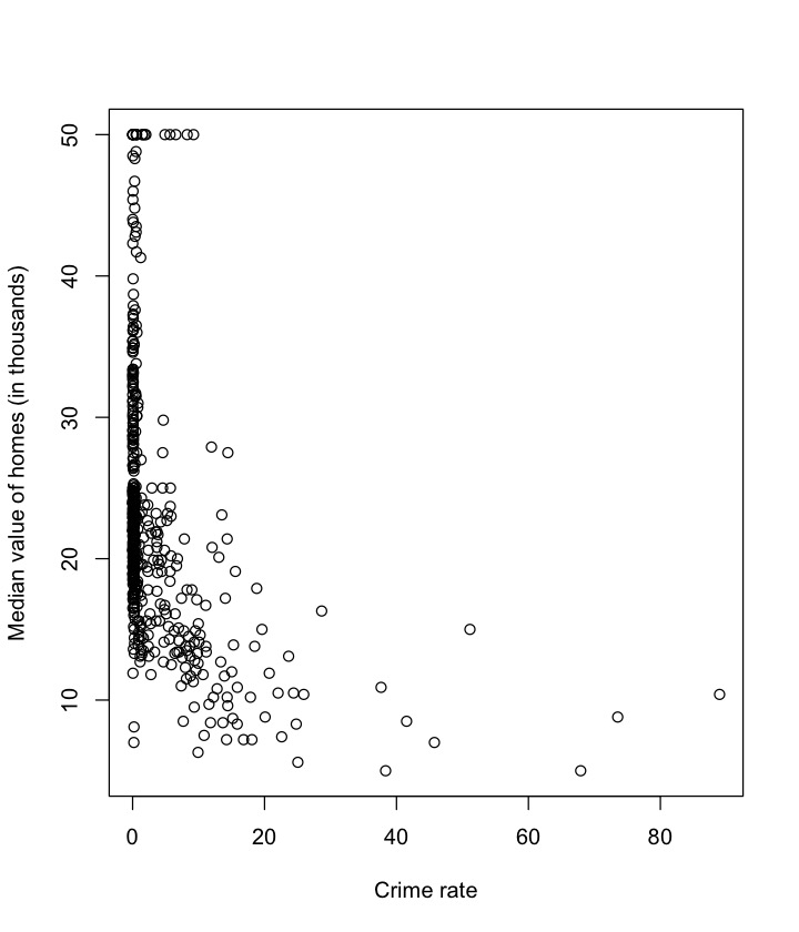
plot(Boston$crim, Boston$medv,
      xlab="Crime rate",
      ylab="Median value of homes (in thousands)")

plot of chunk unnamed-chunk-14

Based on the plot, it seems we should focus on those observations with crim < 25 in plotting.

library(dplyr)
data_subset = tibble(crim=Boston$crim, medv=Boston$medv)
data_subset = filter(data_subset, crim<25)

Here I use the dplyr package which provides some useful “verbs” (functions) for data manipulation. If you use the pipe operator |>, an equivalent (but more readable) way is:

df = as_tibble(Boston) |>
  select(crim, medv) |>
  filter(crim<25)

plot(df$crim, df$medv,
     xlab="Crime rate (less than 25)",
     ylab="Median value of homes (in thousands)")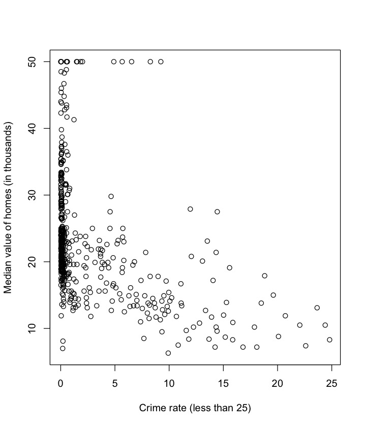

plot of chunk unnamed-chunk-17

Plot each feature against medv:

library(reshape2)
library(ggplot2)
bosmelt <- melt(Boston, id="medv")
ggplot(bosmelt, aes(x=value, y=medv))+
  facet_wrap(~variable, scales="free")+
  geom_point()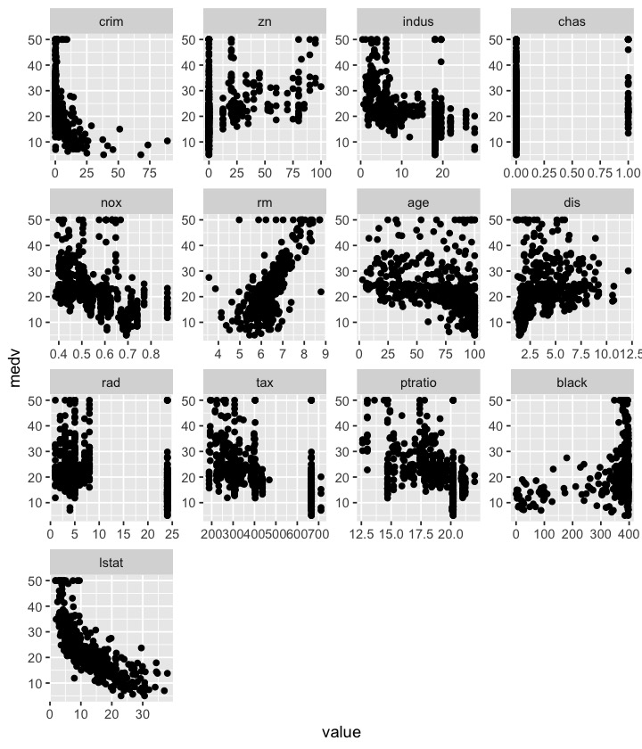

plot of chunk unnamed-chunk-18

Lastly, we compute and visualize the correlation matrix:

corr_m = cor(Boston)
round(corr_m, 2)
#>          crim    zn indus  chas   nox    rm   age   dis   rad   tax ptratio
#> crim     1.00 -0.20  0.41 -0.06  0.42 -0.22  0.35 -0.38  0.63  0.58    0.29
#> zn      -0.20  1.00 -0.53 -0.04 -0.52  0.31 -0.57  0.66 -0.31 -0.31   -0.39
#> indus    0.41 -0.53  1.00  0.06  0.76 -0.39  0.64 -0.71  0.60  0.72    0.38
#> chas    -0.06 -0.04  0.06  1.00  0.09  0.09  0.09 -0.10 -0.01 -0.04   -0.12
#> nox      0.42 -0.52  0.76  0.09  1.00 -0.30  0.73 -0.77  0.61  0.67    0.19
#> rm      -0.22  0.31 -0.39  0.09 -0.30  1.00 -0.24  0.21 -0.21 -0.29   -0.36
#> age      0.35 -0.57  0.64  0.09  0.73 -0.24  1.00 -0.75  0.46  0.51    0.26
#> dis     -0.38  0.66 -0.71 -0.10 -0.77  0.21 -0.75  1.00 -0.49 -0.53   -0.23
#> rad      0.63 -0.31  0.60 -0.01  0.61 -0.21  0.46 -0.49  1.00  0.91    0.46
#> tax      0.58 -0.31  0.72 -0.04  0.67 -0.29  0.51 -0.53  0.91  1.00    0.46
#> ptratio  0.29 -0.39  0.38 -0.12  0.19 -0.36  0.26 -0.23  0.46  0.46    1.00
#> black   -0.39  0.18 -0.36  0.05 -0.38  0.13 -0.27  0.29 -0.44 -0.44   -0.18
#> lstat    0.46 -0.41  0.60 -0.05  0.59 -0.61  0.60 -0.50  0.49  0.54    0.37
#> medv    -0.39  0.36 -0.48  0.18 -0.43  0.70 -0.38  0.25 -0.38 -0.47   -0.51
#>         black lstat  medv
#> crim    -0.39  0.46 -0.39
#> zn       0.18 -0.41  0.36
#> indus   -0.36  0.60 -0.48
#> chas     0.05 -0.05  0.18
#> nox     -0.38  0.59 -0.43
#> rm       0.13 -0.61  0.70
#> age     -0.27  0.60 -0.38
#> dis      0.29 -0.50  0.25
#> rad     -0.44  0.49 -0.38
#> tax     -0.44  0.54 -0.47
#> ptratio -0.18  0.37 -0.51
#> black    1.00 -0.37  0.33
#> lstat   -0.37  1.00 -0.74
#> medv     0.33 -0.74  1.00

library(corrplot) ## visualizing the corr matrix
corrplot(corr_m)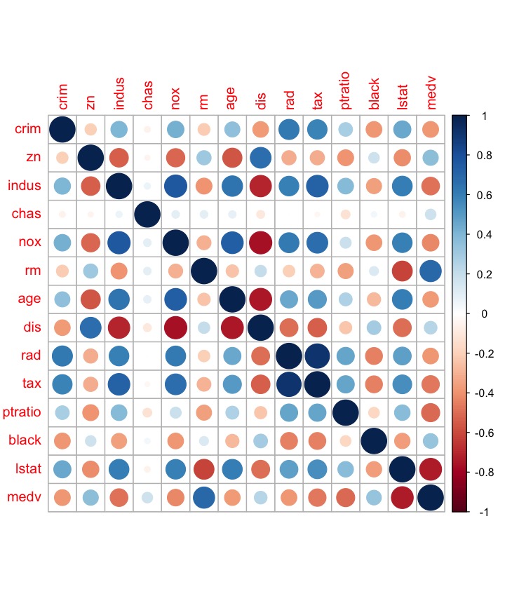

plot of chunk unnamed-chunk-20

Linear regression

We use the lm() function for running linear regression. For example, the syntax lm(y ~ x1 + x2 + x3, data) fits a model with three predictors: $y = \beta_0 + \beta_1 x_1 + \beta_2 x_2 + \beta_3 x_3$ .

Here the Boston dataset contains 13 variables. You can manually specify all the 13 regressors. Fortunately, R provides the short-hand . for performing a regression using all of the predictors:

fit_all = lm(medv ~ ., data = Boston)

As discussed above, fit_all is a list containing all the regression info. The

summary(fit_all)
#> 
#> Call:
#> lm(formula = medv ~ ., data = Boston)
#> 
#> Residuals:
#>     Min      1Q  Median      3Q     Max 
#> -15.595  -2.730  -0.518   1.777  26.199 
#> 
#> Coefficients:
#>               Estimate Std. Error t value Pr(>|t|)    
#> (Intercept)  3.646e+01  5.103e+00   7.144 3.28e-12 ***
#> crim        -1.080e-01  3.286e-02  -3.287 0.001087 ** 
#> zn           4.642e-02  1.373e-02   3.382 0.000778 ***
#> indus        2.056e-02  6.150e-02   0.334 0.738288    
#> chas         2.687e+00  8.616e-01   3.118 0.001925 ** 
#> nox         -1.777e+01  3.820e+00  -4.651 4.25e-06 ***
#> rm           3.810e+00  4.179e-01   9.116  < 2e-16 ***
#> age          6.922e-04  1.321e-02   0.052 0.958229    
#> dis         -1.476e+00  1.995e-01  -7.398 6.01e-13 ***
#> rad          3.060e-01  6.635e-02   4.613 5.07e-06 ***
#> tax         -1.233e-02  3.760e-03  -3.280 0.001112 ** 
#> ptratio     -9.527e-01  1.308e-01  -7.283 1.31e-12 ***
#> black        9.312e-03  2.686e-03   3.467 0.000573 ***
#> lstat       -5.248e-01  5.072e-02 -10.347  < 2e-16 ***
#> ---
#> Signif. codes:  0 '***' 0.001 '**' 0.01 '*' 0.05 '.' 0.1 ' ' 1
#> 
#> Residual standard error: 4.745 on 492 degrees of freedom
#> Multiple R-squared:  0.7406, Adjusted R-squared:  0.7338 
#> F-statistic: 108.1 on 13 and 492 DF,  p-value: < 2.2e-16

Here the summary output still contains lots of info. We can use summary(fit)$r.sq to see the $R^2$ .

summary(fit_all)$r.sq ## short for summary(fit_all)[["r.sq"]]
#> [1] 0.7406427

Excluding certain predictors

From the summary, age and indus seem to have high p-values.

We can run a regression excluding these two predictors:

fit_ex = lm(medv ~ . - age - indus, data=Boston)

summary(fit_ex)
#> 
#> Call:
#> lm(formula = medv ~ . - age - indus, data = Boston)
#> 
#> Residuals:
#>      Min       1Q   Median       3Q      Max 
#> -15.5984  -2.7386  -0.5046   1.7273  26.2373 
#> 
#> Coefficients:
#>               Estimate Std. Error t value Pr(>|t|)    
#> (Intercept)  36.341145   5.067492   7.171 2.73e-12 ***
#> crim         -0.108413   0.032779  -3.307 0.001010 ** 
#> zn            0.045845   0.013523   3.390 0.000754 ***
#> chas          2.718716   0.854240   3.183 0.001551 ** 
#> nox         -17.376023   3.535243  -4.915 1.21e-06 ***
#> rm            3.801579   0.406316   9.356  < 2e-16 ***
#> dis          -1.492711   0.185731  -8.037 6.84e-15 ***
#> rad           0.299608   0.063402   4.726 3.00e-06 ***
#> tax          -0.011778   0.003372  -3.493 0.000521 ***
#> ptratio      -0.946525   0.129066  -7.334 9.24e-13 ***
#> black         0.009291   0.002674   3.475 0.000557 ***
#> lstat        -0.522553   0.047424 -11.019  < 2e-16 ***
#> ---
#> Signif. codes:  0 '***' 0.001 '**' 0.01 '*' 0.05 '.' 0.1 ' ' 1
#> 
#> Residual standard error: 4.736 on 494 degrees of freedom
#> Multiple R-squared:  0.7406, Adjusted R-squared:  0.7348 
#> F-statistic: 128.2 on 11 and 494 DF,  p-value: < 2.2e-16

Interaction and nonlinear terms

The syntax lstat:black tells R to include the interaction term $\text{lstat}\times\text{black}$ .
The syntax lstat*age simultaneously include lstat, age, and the interaction term lstat:black as predictors:

summary(lm(medv ~ lstat*age, data=Boston))
#> 
#> Call:
#> lm(formula = medv ~ lstat * age, data = Boston)
#> 
#> Residuals:
#>     Min      1Q  Median      3Q     Max 
#> -15.806  -4.045  -1.333   2.085  27.552 
#> 
#> Coefficients:
#>               Estimate Std. Error t value Pr(>|t|)    
#> (Intercept) 36.0885359  1.4698355  24.553  < 2e-16 ***
#> lstat       -1.3921168  0.1674555  -8.313 8.78e-16 ***
#> age         -0.0007209  0.0198792  -0.036   0.9711    
#> lstat:age    0.0041560  0.0018518   2.244   0.0252 *  
#> ---
#> Signif. codes:  0 '***' 0.001 '**' 0.01 '*' 0.05 '.' 0.1 ' ' 1
#> 
#> Residual standard error: 6.149 on 502 degrees of freedom
#> Multiple R-squared:  0.5557, Adjusted R-squared:  0.5531 
#> F-statistic: 209.3 on 3 and 502 DF,  p-value: < 2.2e-16

To include the quadratic term X^2, use I(X^2):

The special function I() is needed since the hat symbol ^ has a special meaning in a formula.

fit_nonlinear = lm(medv~lstat+I(lstat^2), data = Boston)
summary(fit_nonlinear)
#> 
#> Call:
#> lm(formula = medv ~ lstat + I(lstat^2), data = Boston)
#> 
#> Residuals:
#>      Min       1Q   Median       3Q      Max 
#> -15.2834  -3.8313  -0.5295   2.3095  25.4148 
#> 
#> Coefficients:
#>              Estimate Std. Error t value Pr(>|t|)    
#> (Intercept) 42.862007   0.872084   49.15   <2e-16 ***
#> lstat       -2.332821   0.123803  -18.84   <2e-16 ***
#> I(lstat^2)   0.043547   0.003745   11.63   <2e-16 ***
#> ---
#> Signif. codes:  0 '***' 0.001 '**' 0.01 '*' 0.05 '.' 0.1 ' ' 1
#> 
#> Residual standard error: 5.524 on 503 degrees of freedom
#> Multiple R-squared:  0.6407, Adjusted R-squared:  0.6393 
#> F-statistic: 448.5 on 2 and 503 DF,  p-value: < 2.2e-16

The near-zero p-value associated with the quadratic term suggests that it leads to an improved model.

Review questions

What’s the difference between vector and list? Explain in your own words.
m = matrix(1:4, nrow = 2). Is m a vector or a list?
Is the dataset Boston a vector or a list?

Read about the dataset (?Boston) and answer the following questions.

How to know the number of rows and columns in dataset Boston?
Make some pairwise scatterplots of the predictors (columns) in this data set. Describe your findings.
Are any of the predictors associated with crim (per capita crime rate)? If so, explain the relationship.
Do any of the suburbs of Boston appear to have particularly high crime rates? Tax rates? Pupil-teacher ratios? Comment on the range of each predictor.
How many of the suburbs in this data set bound the Charles river?

Colophon. This document is built with Pandoc and Knitr, with the following knitr setup:

knitr::opts_chunk$set(collapse = TRUE, comment = "#>")