To install R, read the official cran page, which provides detailed instructions regarding how to install R on different operating systems (Linux, macOS and Windows).
RStudio is a great environment for writing and executing R scripts in this course. You can download RStudio freely from its official page.
If you are new to programming, I recommend RStudio as it works outside of the box. You already have everything you need for this course after installing R and RStudio.
R creates an interactive environment for you to play with data and statistical models. If you have no exposure to computer-based statistical computing before, I dare say that learning R will be the most valuable experience for you in this course.
After installing R and RStudio on your computer, you can play with the following scripts in RStudio. There are three ways to run R code in RStudio:
Use the R console. By default, it should be the left-bottom sub-window of RStudio.
Write your R scripts in the code editor (it should be the
left-top sub-window). Then, run your R Scripts line by line using the
shortcut Ctrl-Enter/Command-Enter (or maybe
Shift-Enter, depending on whether your are using windows,
mac or Linux).
Write your R Scripts in Quarto. Indeed, this guide is written in Quarto. You can find the Quarto source by following the link in the index page.
## In R, comments start with ## symbol
## This line will not be run
Note: This document is generated by knitr, and
outputs of each code chunk are automatically generated and included with
the #> prefix.
num = 3
num + 2
#> [1] 5

### vector
x = c(2, 7, 5) ## Here "c" is short for combine
x
#> [1] 2 7 5

### a vector (sequence) from 1 to 5
y = seq(1, 5)
y
#> [1] 1 2 3 4 5

### a sequence from 1 to 5, with each step increasing by 2
seq(1, 5, 2) ## seq(from=1, to=5, by=2)
#> [1] 1 3 5

x + y
#> Warning in x + y: longer object length is not a multiple of shorter object
#> length
#> [1]  3  9  8  6 12
Run ?seq to read the manual of the seq
function.
x / y
#> Warning in x/y: longer object length is not a multiple of shorter object length
#> [1] 2.000000 3.500000 1.666667 0.500000 1.400000

### extracting sub-vector (also called subsetting)
x[1]
#> [1] 2
c(x[1], x[3])
#> [1] 2 5
x[1:3] ## same as x as length(x) == 3
#> [1] 2 7 5
length(x)
#> [1] 3
x[-1]
#> [1] 7 5
### matrix
z = matrix(seq(1,12), nrow= 3)
z
#> [,1] [,2] [,3] [,4]
#> [1,] 1 4 7 10
#> [2,] 2 5 8 11
#> [3,] 3 6 9 12
dim(z)
#> [1] 3 4
length(z)
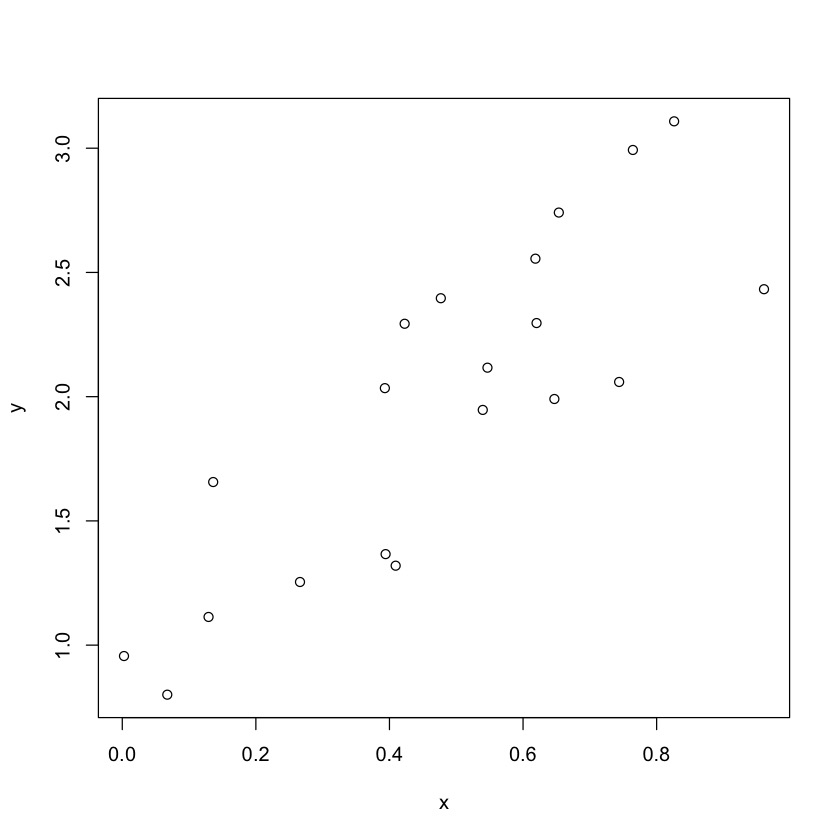
#> [1] 12set.seed(2020)
x = runif(20)
x
#> [1] 0.646902839 0.394225758 0.618501814 0.476891136 0.136097186 0.067384386
#> [7] 0.129152617 0.393117930 0.002582699 0.620205954 0.764414018 0.743835758
#> [13] 0.826165695 0.422729083 0.409287665 0.539692614 0.960722398 0.653557334
#> [19] 0.546715299 0.266063566
e = runif(20)
y = 0.5 + x * 2 + e
plot(x,y)
The function lm() is for fitting linear models. Here we
simply regress y on x.
First, we create a dataframe for our generated data:
my_data = data.frame(y = y, x = x)my_lm = lm(y ~ x, data = my_data)
summary(my_lm)
#>
#> Call:
#> lm(formula = y ~ x, data = my_data)
#>
#> Residuals:
#> Min 1Q Median 3Q Max
#> -0.56217 -0.30050 0.00473 0.40064 0.44601
#>
#> Coefficients:
#> Estimate Std. Error t value Pr(>|t|)
#> (Intercept) 0.946 0.176 5.374 4.16e-05 ***
#> x 2.132 0.323 6.602 3.36e-06 ***
#> ---
#> Signif. codes: 0 '***' 0.001 '**' 0.01 '*' 0.05 '.' 0.1 ' ' 1
#>
#> Residual standard error: 0.3703 on 18 degrees of freedom
#> Multiple R-squared: 0.7077, Adjusted R-squared: 0.6915
#> F-statistic: 43.59 on 1 and 18 DF, p-value: 3.362e-06my_lm["coefficients"]
#> $coefficients
#> (Intercept) x
#> 0.9459971 2.1324126
## To know other options besides coefficients, run
## str(my_lm)
## Also, try running:
## my_lm$coefficients#create scatterplot
plot(y ~ x, data=my_data)
#add fitted regression line to scatterplot
abline(my_lm)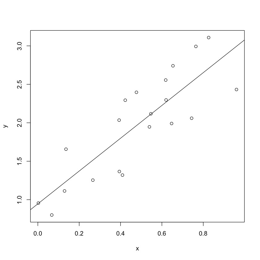
Base R is powerful enough for many routine statistical tasks. You can also use third-party R packages to make your work easier.
ggplot2 is a package for plotting, which
provides a more sophisticated layout than the base plot()
function:
## install ggplot2. You only need to do it once.
install.packages("ggplot2")library(ggplot2)
#create scatterplot with fitted regression line
ggplot(my_data, aes(x = x, y = y)) +
geom_point() +
stat_smooth(method = "lm", se=FALSE)
#> `geom_smooth()` using formula = 'y ~ x'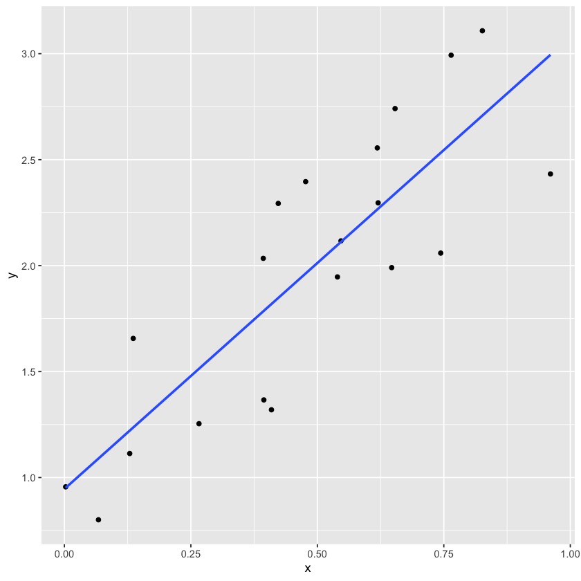
You should have a basic understanding about using R now. For further knowledge, I recommend the following materials:
How do you create a vector in R?
Given a vector x, how to get its length?
How to create a vector in R?
Given x=c(1,2,3) and y=c(1,5), what’s
x-y?
Given a vector x, how do you get its third element?
What if length(x) == 2?
How do you generate a sequence where each ?
what’s a seed? Why do we use
set.seed(2020)?
Given a data set data with two variables
x and y, how do you fit the linear model
?
Explain the output of summary(my_lm) in our
example:
Call:
lm(formula = y ~ x, data = my_data)

Residuals:
     Min       1Q   Median       3Q      Max
-0.56217 -0.30050  0.00473  0.40064  0.44601

Coefficients:
            Estimate Std. Error t value Pr(>|t|)
(Intercept)    0.946      0.176   5.374 4.16e-05 ***
x              2.132      0.323   6.602 3.36e-06 ***
---
Signif. codes:  0 '***' 0.001 '**' 0.01 '*' 0.05 '.' 0.1 ' ' 1

Residual standard error: 0.3703 on 18 degrees of freedom
Multiple R-squared:  0.7077,    Adjusted R-squared:  0.6915
F-statistic: 43.59 on 1 and 18 DF,  p-value: 3.362e-06
Colophon. This document is built with Pandoc and Knitr, with the following knitr setup:
knitr::opts_chunk$set(collapse = TRUE, comment = "#>")